Pun intended.

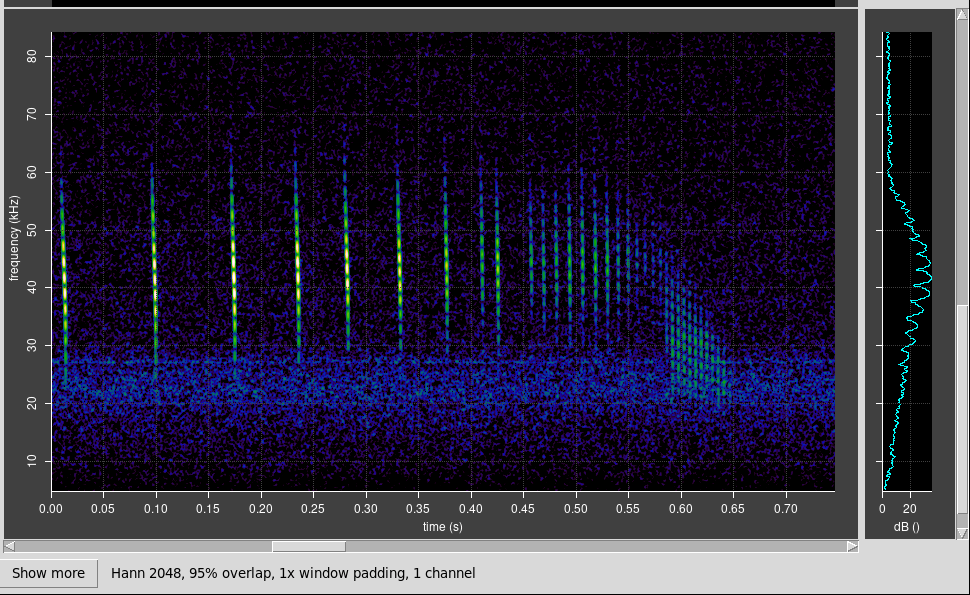
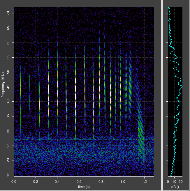
It’s common to see bright and dark bands in spectrograms of bats flying close to reflective surfaces. Typically, they are seen with Daubenton’s bats flying low over water, but can also seen with any bat species flying near a reflective surface, when the resulting echo overlaps the original chirp.

The explanation is straightforward. Sound from the bat arrives at the microphone via two different paths – the direct path, and the path reflected from the surface. The result is wave interference. If the sound arrives in phase via the two paths at a detector, the sound is reinforced and results in a brighter region in the spectrogram. If it arrives in antiphase, the sound largely cancels out, resulting in a darker region. Intermediate phase differences result in intermediate degrees of reinforcement or cancellation.

Banding is only visible in the spectrogram when the original chirp and echo are so close that they overlap in spectrogram. If they are separated in the spectrogram, banding is not visible, but the effect still results in a visible modulation in the signal amplitude graph. See the examples on the left of this page.

The phase difference between sound waves arriving via the two paths depends on multiple factors, including

• The difference in length of the direct and reflected paths.
• The frequency.
• Changes in the frequency.
• Doppler effect.

I will concentrate on the first of these factors, the path difference, and briefly discuss the other factors at the end.

Calculation of Path Difference

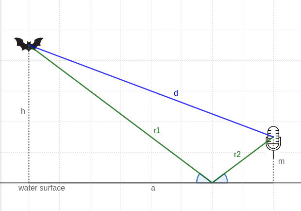
The diagram shows a bat flying at height h over a reflective surface, being detected by a microphone at height m, at a distance a. Sound waves arrive at the microphone via a direct path d, and by a reflected path (r1 + r2). We are interested in the difference in length of those two paths, as this will translate to phase difference. I’ve deliberately drawn a diagram that makes it clear that the direct path need not be parallel to the surface of the water, nor the bat very close to the water.

The length of the direct path is easy – Pythagoras tells us the answer without further ado. The length of the reflected path is more complex. It is in two parts which we need to sum. To apply Pythagoras we need to know the distance of the point of reflection from the microphone. This could be calculated using some trigonometry, then r1 and r2 calculated, and added.

That can certainly be done. However there is a trick that makes this much simpler. When a sound wave is reflected, the angle of incidence is equal to the angle of reflection. These two equal angles are shown the diagram above. The trick we will use is to flip over the left hand triangle, formed of h and r1, without making any other change to it. Think of it as reflecting the triangle in the surface of the water. Here’s a version of the diagram with flipped triangle added:

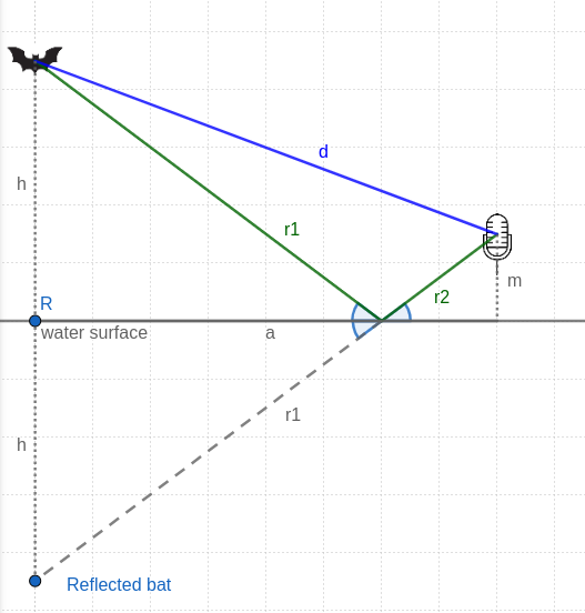
Here’s the thing. All the angles indicated in the diagram are now equal. That means that r2 and the reflection of r1 are in a straight line (vertically opposite angles). The total of r1 + r2 can now be straightforwardly calculated using Pythagoras, as for the direct path. In other words, the reflected path is just the distance from the reflection of the bat in the water to the real microphone above the water.

Here is some maths to make it respectable, complete with a Greek letter for additional plausibility. The length of the direct path from the real bat to the real microphone is

Likewise, the total length of the reflected path reflected bat to the real microphone is:

Note that the only difference is the change of sign. The path difference Δ is then just:

Good, now we have the path difference. But we really want the phase difference, or more specifically, to know if the direct path and reflected path sounds reinforce or cancel each other. The two paths will reinforce when the path difference is an exact multiple of the wavelength of the bat chirp. In other words, they will reinforce when:

where n is a whole number, c is the speed of sound (343 m/s) and f is the frequency. The frequency spacing of the bands is the difference between successive frequencies that result in reinforcement of sound. Those frequencies corresponding to adjacent band maxima, f₁ and f₂, satisfying this relation:

Cancelling c and rearranging to get Δf, the frequency difference between f₁ and f₂

So finally we have it: the spacing of bands depends on the number of wavelengths of sound that fit in the path difference. This is equivalent to the number of cycles in the echo delay time.

Plugging in some realistic numbers for illustration: if the bat is 0.3 m above the water, the microphone is 1 m above the water and bat is 5 m away, the path difference would be 0.12 m. At 45 kHz, that corresponds to about 16 wavelengths of sound (n = 16), and the band spacing would be about 2.8 kHz. That is similar to what is observed. However, it’s pretty hard to know the bat’s height and distance away at any instant.

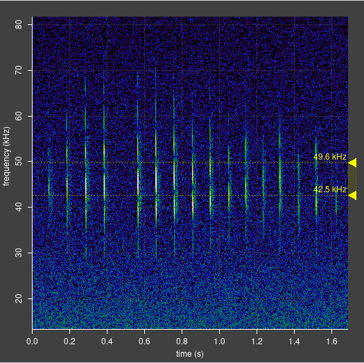
Approaching it a different way, based on the Daubenton bat spectrograms above, the echo delay measured from the spectrogram just before the feeding buzz is about 0.5 ms. At 45 kHz, that’s about 22 cycles, so there are 22 wavelengths of sound in the path difference (n = 22). The predicted band spacing around 45 kHz, by the formula above, is about 2 kHz (45,000 / 22). Measured from the spectrogram, the band spacing is actually 2.5 kHz, which is fairly close, but not exactly what we predict.

Interestingly, the band spacing is independent of frequency, which cancels out of the calculations. This is in fact what is observed in reality.

Other Factors

Based on the difference in length between the direct and reflected sound path, we did some maths and made some predictions that weren’t too far from reality. However, the predictions didn’t exactly match reality. What’s going on?

Well, we solved the problem of the ideal bat – motionless, and emitting a constant frequency. Can you tell my degree was physics? However, real bats are moving pretty fast, and their chirps are far from constant in frequency.

Speed of motion of the bat results in a shift in the apparent frequency of the bat chirp due to the Doppler effect.. For example, a bat emitting 45 kHz, and flying directly towards an observer, would have an apparent frequency of 45.67 kHz because of the Doppler shift. So, can we just use all the formulae above substituting a value of 45.67 kHz? Not quite. The issue is that the reflected bat is travelling directly towards the reflected microphone, not the real microphone. It approaches the real microphone at an angle that results in somewhat less Doppler shift. That makes quite a small difference in the equations above, so the assumption of a stationary bat is not too bad.

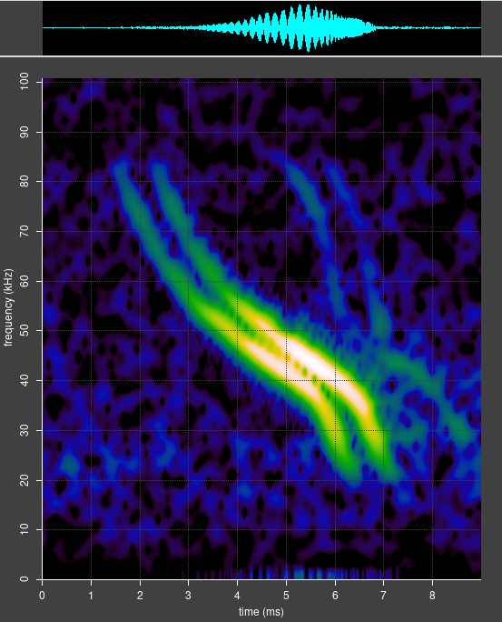
The other assumption we made is more problematic. We assumed the bat was emitting a constant frequency. But looking at a specific Daubenton’s bat chirp in the data used, there is a sweep from 83kHz down to 21 kHz in about 5ms – an average of around 12 kHz per ms. That means that the chirp arriving via the longer reflected path is about 6 kHz higher in frequency than the chirp arriving via the direct path. A correction would need to be made to the calculations above – though in practice, the effect seems to be small.

Conclusion

We modelled the direct and reflected sound paths for an ideal bat being detected by a microphone and came up with some predictions about band spacing that were close to reality, but not exactly matching. Further consideration suggests that for bats with rapidly sweeping chirps, we need some more complex analysis, or perhaps a simple simulation in code. For bats with relatively constant chirps or parts of chirps (qCF), the simple analysis above should suffice.

Appendix – Band Spacing Predictions

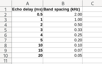
It’s straightforward to create a spreadsheet that predicts band spacing from echo delay for the ideal bat, ie slow moving bats with qCF chirps:

Appendix – Simulation of Banding

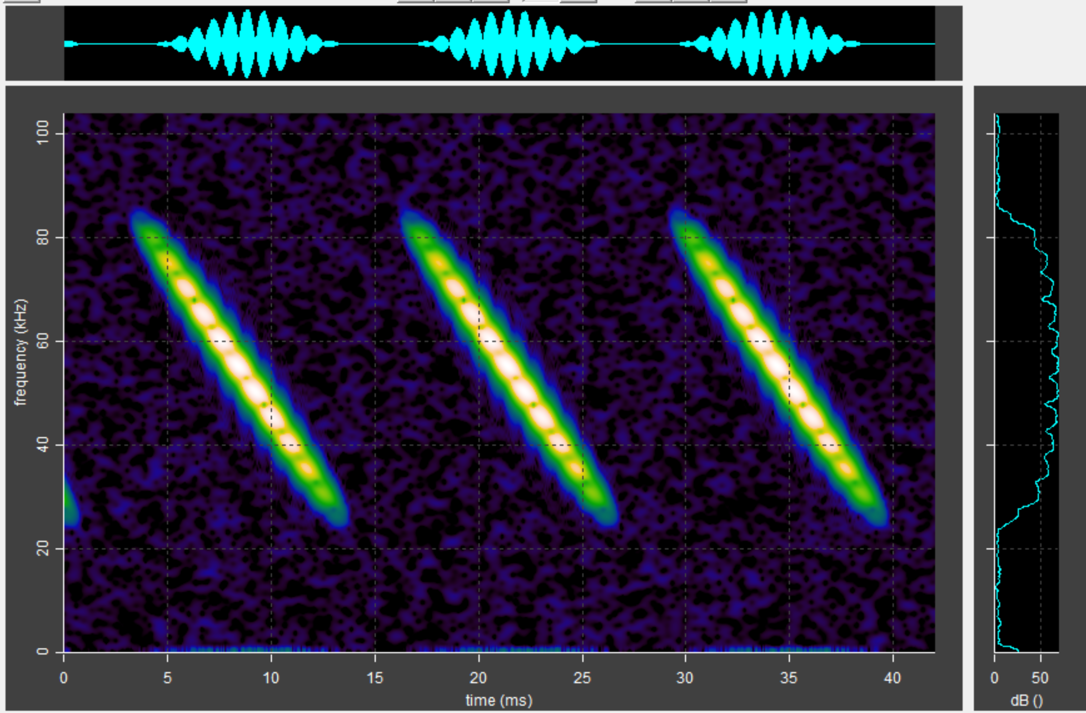
The Python programming language, together with libraries such as numpy, is convenient for audio simulations and creation of wav files. I wrote a simple program that generates a series of linear chirps ranging from 85 to 25 kHz over 10 ms (so something like a Daubenton echolocation call), and simulates a reflected path by adding in a second slightly delayed copy of the same chirps. The result is as predicted by the analysis above: an echo delay of 0.2 ms results in banding of 5 kHz separation.

import wave
import numpy as np

sample_rate = 384000                    # per second
total_samples = int(sample_rate * 0.5)
noise_amplitude = 16

chirp_duration = 0.01                   # seconds
chirp_start = 85000                     # Hz
chirp_end = 25000                       # Hz

echo_delay = 0.0002                     # seconds

wav_file = wave.open("output.wav", "wb")
wav_file.setnchannels(1)
wav_file.setsampwidth(2)
wav_file.setframerate(sample_rate)

# Initialize the data with background noise:
data = np.random.normal(0, noise_amplitude, size=total_samples).astype(np.int16)

# Create a chirp. Note the factor of 1/2 applied to the frequency which is a result
# of the resultant frequency (rate of change of phase) being a product of two variables
# (time and frequency). Remember the product rule from calculus?
chirp_times = np.linspace(0, chirp_duration, num=int(sample_rate * chirp_duration))
chirp_frequencies = chirp_start + chirp_times * (chirp_end - chirp_start) / (2 * chirp_duration)
chirp_data = np.sin(2 * np.pi * chirp_frequencies * chirp_times) * 10000
chirp_data *= np.hanning(len(chirp_data))       # Window the chirp to avoid abrupt starts and ends.
chirp_len = len(chirp_data)

# Copy some chirps into the data, with a time offset:
delay_samples = int(echo_delay * sample_rate)
for pos in range(0, total_samples - chirp_len, int(chirp_len * 1.3)):
    data[pos:pos+chirp_len] += chirp_data.astype(np.int16)
    data[pos+delay_samples:pos+chirp_len+delay_samples] += chirp_data.astype(np.int16)

# Write a wave file:
wav_file.writeframes(data)

Appendix – the Parable of the Ideal Horse

There was once a very rich man who owned race horses and strongly wished to win races. His horses were good, but they didn’t win as often as he wanted them do. To a rich man, this problem can be solved. He commissioned three teams to come up with a horse that would win races, and gave each team a large sum of money to pay for their work. The first team consisted of biologists, the second team consisted of engineers, and the third team consisted of physicists. He gave each team one year to come up with a horse that would win races.

After the year had elapsed, the rich man returned to the teams to see what they had come up with.

The biologists had done some highly accelerated horse breeding. Their horse was very large, very muscular, and pawing at the ground ready to run. The rich man was pleased with their work.

The engineers had come up with a gleaming stainless steel horse, containing an rocket engine, aerodynamically shaped, and powered by liquid hydrogen and oxygen. Surely this was the winning horse.

Finally, the rich man visited the physicists. He couldn’t see any kind of horse, but the physicists were busy writing in their notebooks, brows furrowed, ignoring him. This was confusing. Finally he broke the silence and asked them what the result of their year’s work was. The physicist nearest him replied, “well, sir, we have nearly solved the problem of the spherical horse”.

[Credit for this parable to Mr Dunn, my O level maths teacher, 1979.]